

Viterbi Algorithm
Following Section 5.3.3.2 of [Müller, FMP, Springer 2015], we describe in this notebook the Viterbi algorithm, which efficiently solves the uncovering problem of hidden Markov models (HMMs). For a detailed introduction of HMMs, we refer to the famous tutorial paper by Rabiner.
-
Lawrence R. Rabiner: A Tutorial on Hidden Markov Models and Selected Applications in Speech Recognition. Proceedings of the IEEE, 77 (1989), pp. 257–286.
Bibtex
Uncovering Problem and Viterbi Algorithm
We now consider the uncovering problem, which is the problem relevant for our chord recognition scenario, in more detail. As described in the FMP notebook on Hidden Markov Models (HMMs), the goal is to find the single state sequence $S=(s_{1},s_{2},\ldots,s_{N})$ that "best explains" a given observation sequence $O=(o_{1},o_{2},\ldots,o_{N})$. In the chord recognition scenario, the observation sequence is a sequence of chroma vectors extracted from an audio recording. The optimal state sequence is then the sequence of chord labels, which is the result of the chord recognition procedure. As optimization criterion, one possibility is to choose the state sequence $S^\ast$ that yields the highest probability $\mathrm{Prob}^\ast$ when evaluated against the observation sequence $O$:
\begin{eqnarray} \mathrm{Prob}^\ast &=& \underset{S=(s_{1},s_{2},\ldots,s_{N})}{\max} \,\,P[O,S|\Theta],\\ S^\ast &=& \underset{S=(s_{1},s_{2},\ldots,s_{N})}{\mathrm{argmax}} \,\,\,P[O,S|\Theta]. \end{eqnarray}To find the sequence $S^\ast$ using the naive approach, one would have to compute the probability value $P[O,S|\Theta]$ for each of the $I^N$ possible state sequences of length $N$ and then look for the maximizing argument. Fortunately, there is a technique known as the Viterbi algorithm for finding the optimizing state sequence in a much more efficient way. The Viterbi algorithm, which is similar to the DTW algorithm, is based on dynamic programming. The idea is to recursively compute an optimal (i.e., probability-maximizing) state sequence from optimal solutions for subproblems, where one considers truncated versions of the observation sequence. Let $O=(o_{1},o_{2},\ldots o_{N})$ be the observation sequence. Then, we define the prefix
$$ O(1\!:\!n):=(o_{1},\ldots,o_{n}) $$of length $n\in[1:N]$ and set
\begin{equation} \mathbf{D}(i,n):=\underset{(s_1,\ldots,s_n)}{\max} P[O(1:n),(s_1,\ldots, s_{n-1},s_n=\alpha_i)|\Theta] \end{equation}for $i\in[1:I]$. In other words, $\mathbf{D}(i,n)$ is the highest probability along a single state sequence $(s_{1},\ldots,s_{n})$ that accounts for the first $n$ observations and ends in state $s_{n}=\alpha_{i}$. The state sequence yielding the maximal value
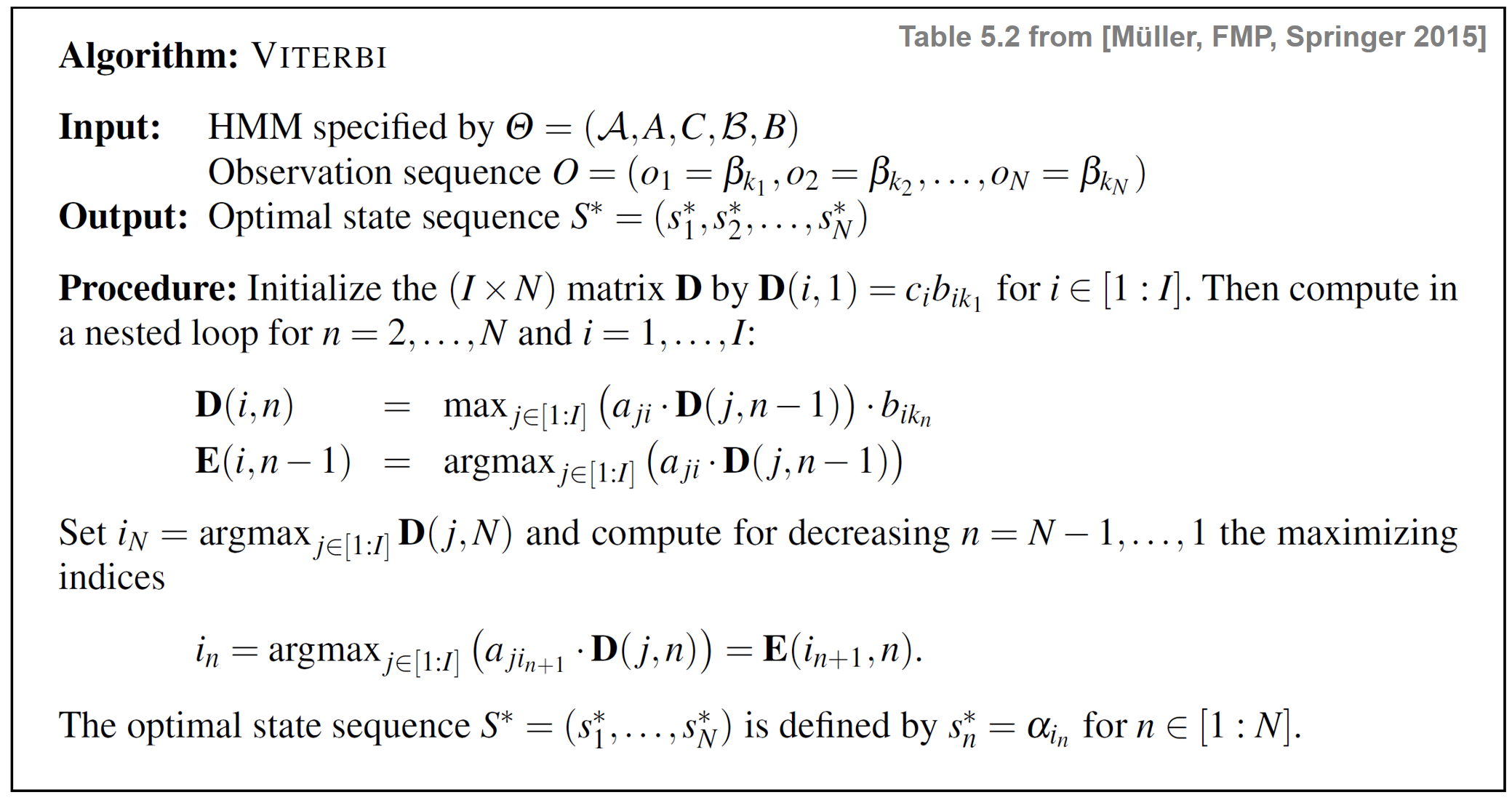
\begin{equation} \label{eq:ChordReco:HMM:Problems:UncovMax} \mathbf{Prob}^\ast = \underset{i\in[1:I]}{\max}\,\,\mathbf{D}(i,N) \end{equation}is the solution to our uncovering problem. The $(I\times N)$ matrix $\mathbf{D}$ can be computed recursively along the column index $n\in[1:N]$. The following table specifies the Viterbi algorithm. For a detailed explanation of the algorithm, we refer to Section 5.3.3.2 of [Müller, FMP, Springer 2015].
The following figure illustrates the main steps of the Viterbi algorithm.
- The blue cells indicate the entries $\mathbf{D}(i,1)$, which serve as initialization of the algorithm.
- The red cells illustrate the computation of the main iteration.
- The black cell indicates the maximizing index used for the back tracking to obtain the optimal state sequence.
- The matrix $E$ is used to keep track of the maximizing indices in the recursion. This information is needed in the second stage when constructing the optimal state sequence using backtracking.
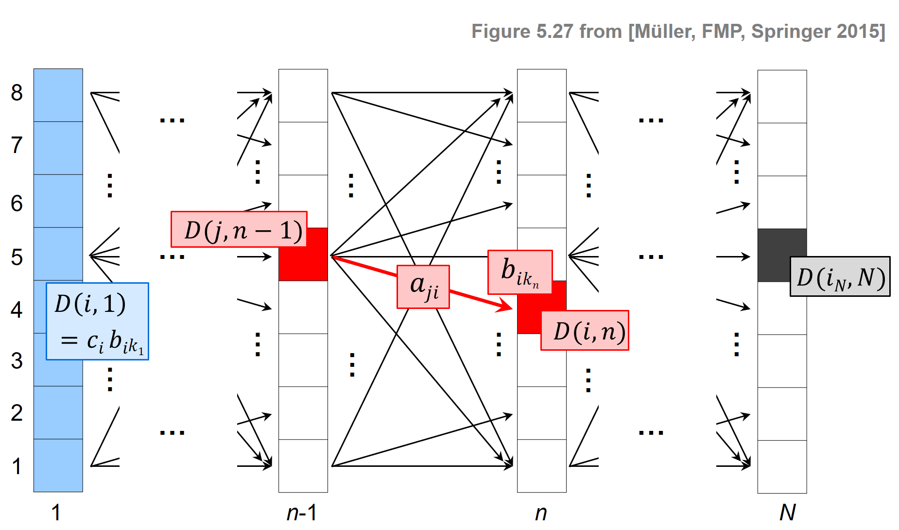
The overall procedure is similar to the DTW algorithm, where one first constructs the accumulated cost matrix and then obtains the optimal warping path using backtracking. As illustrated by the previous figure, the Viterbi algorithm proceeds in an iterative fashion building up a graph-like structure with $N$ layers, each consisting of $I$ nodes (the states). Furthermore, two neighboring layers are connected by $I^2$ edges, which also determines the order of the number of operations needed to construct a new layer from a given layer. From this follows that the computational complexity of the Viterbi algorithm is $O(N\cdot I^2)$, which is much better than $O(I^N)$ required for the naive approach.
Toy Example
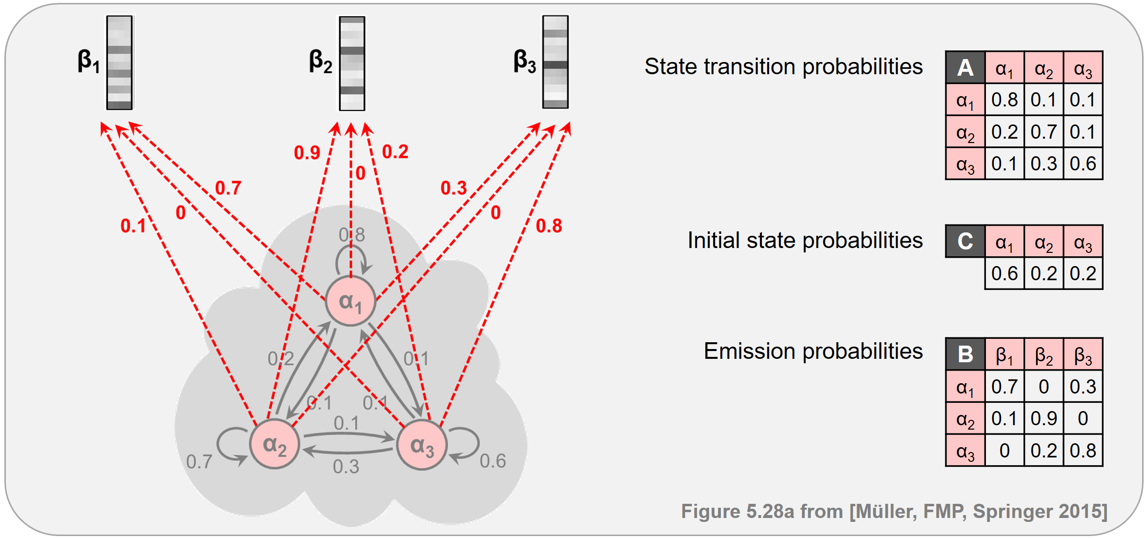
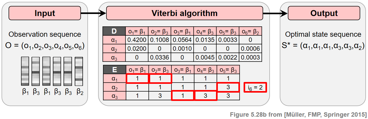
Continuing our toy example from the FMP notebook on HMMs, the next figure illustrates the principle of the Viterbi algorithm. At the top, one finds a specification of the HMM. At the bottom, the Viterbi algorithm is applied for an input sequence of length $N=6$.
Implementation of Viterbi Algorithm
In the next code cell, we provide an implementation of the Viterbi algorithm.
0. Also, there is an index shift when applying the algorithm to our toy example, which becomes O = [0, 2, 0, 2, 2, 1].
import numpy as np
from numba import jit

@jit(nopython=True)
def viterbi(A, C, B, O):
    """Viterbi algorithm for solving the uncovering problem

    Notebook: C5/C5S3_Viterbi.ipynb

    Args:
        A (np.ndarray): State transition probability matrix of dimension I x I
        C (np.ndarray): Initial state distribution  of dimension I
        B (np.ndarray): Output probability matrix of dimension I x K
        O (np.ndarray): Observation sequence of length N

    Returns:
        S_opt (np.ndarray): Optimal state sequence of length N
        D (np.ndarray): Accumulated probability matrix
        E (np.ndarray): Backtracking matrix
    """
    I = A.shape[0]    # Number of states
    N = len(O)  # Length of observation sequence

    # Initialize D and E matrices
    D = np.zeros((I, N))
    E = np.zeros((I, N-1)).astype(np.int32)
    D[:, 0] = np.multiply(C, B[:, O[0]])

    # Compute D and E in a nested loop
    for n in range(1, N):
        for i in range(I):
            temp_product = np.multiply(A[:, i], D[:, n-1])
            D[i, n] = np.max(temp_product) * B[i, O[n]]
            E[i, n-1] = np.argmax(temp_product)

    # Backtracking
    S_opt = np.zeros(N).astype(np.int32)
    S_opt[-1] = np.argmax(D[:, -1])
    for n in range(N-2, -1, -1):
        S_opt[n] = E[int(S_opt[n+1]), n]

    return S_opt, D, E

# Define model parameters
A = np.array([[0.8, 0.1, 0.1],
              [0.2, 0.7, 0.1],
              [0.1, 0.3, 0.6]])

C = np.array([0.6, 0.2, 0.2])

B = np.array([[0.7, 0.0, 0.3],
              [0.1, 0.9, 0.0],
              [0.0, 0.2, 0.8]])


O = np.array([0, 2, 0, 2, 2, 1]).astype(np.int32)
#O = np.array([1]).astype(np.int32)
#O = np.array([1, 2, 0, 2, 2, 1]).astype(np.int32)

# Apply Viterbi algorithm
S_opt, D, E = viterbi(A, C, B, O)
#
print('Observation sequence:   O = ', O)
print('Optimal state sequence: S = ', S_opt)
np.set_printoptions(formatter={'float': "{: 7.4f}".format})
print('D =', D, sep='\n')
np.set_printoptions(formatter={'float': "{: 7.0f}".format})
print('E =', E, sep='\n')
Log-Domain Implementation of Viterbi Algorithm
In each iteration of the Viterbi algorithm, the accumulated probability values of $\mathbf{D}$ at step $n-1$ are multiplied with two probability values from $A$ and $B$. More precisely, we have
$$ \mathbf{D}(i,n) = \max_{j\in[1:I]}\big(a_{ij} \cdot\mathbf{D}(j,n-1) \big) \cdot b_{i_{k_n}}. $$Since all probability values lie the interval $[0,1]$, the product of such values decreases exponentially with the number $n$ of iterations. As a result, for input sequences $O=(o_{1},o_{2},\ldots o_{N})$ with large $N$, the values in $\mathbf{D}$ typically become extremely small, which may finally lead to a numerical underflow. A well-known trick when dealing with products of probability values is to work in the log-domain. To this end, one applies a logarithm to all probability values and replaces multiplication by summation. Since the logarithm is a strictly monotonous function, ordering relations are preserved in the log-domain, which allows for transferring operations such as maximization or minimization.
In the following code cell, we provide a log variant of the Viterbi algorithm. This variant yields exactly the same optimal state sequence $S^\ast$ and the same backtracking matrix $E$ as the original algorithm, as well as the accumulated log probability matrix $\log(\mathbf{D})$ (D_log) (where the logarithm is applied for each entry). We again test the implementation on our toy example. Furthermore, as a sanity check, we apply the exponential function to the computed log-matrix D_log, which should yield the matrix D as computed by the original Viterbi algorithm above.
@jit(nopython=True)
def viterbi_log(A, C, B, O):
    """Viterbi algorithm (log variant) for solving the uncovering problem

    Notebook: C5/C5S3_Viterbi.ipynb

    Args:
        A (np.ndarray): State transition probability matrix of dimension I x I
        C (np.ndarray): Initial state distribution  of dimension I
        B (np.ndarray): Output probability matrix of dimension I x K
        O (np.ndarray): Observation sequence of length N

    Returns:
        S_opt (np.ndarray): Optimal state sequence of length N
        D_log (np.ndarray): Accumulated log probability matrix
        E (np.ndarray): Backtracking matrix
    """
    I = A.shape[0]    # Number of states
    N = len(O)  # Length of observation sequence
    tiny = np.finfo(0.).tiny
    A_log = np.log(A + tiny)
    C_log = np.log(C + tiny)
    B_log = np.log(B + tiny)

    # Initialize D and E matrices
    D_log = np.zeros((I, N))
    E = np.zeros((I, N-1)).astype(np.int32)
    D_log[:, 0] = C_log + B_log[:, O[0]]

    # Compute D and E in a nested loop
    for n in range(1, N):
        for i in range(I):
            temp_sum = A_log[:, i] + D_log[:, n-1]
            D_log[i, n] = np.max(temp_sum) + B_log[i, O[n]]
            E[i, n-1] = np.argmax(temp_sum)

    # Backtracking
    S_opt = np.zeros(N).astype(np.int32)
    S_opt[-1] = np.argmax(D_log[:, -1])
    for n in range(N-2, -1, -1):
        S_opt[n] = E[int(S_opt[n+1]), n]

    return S_opt, D_log, E

# Apply Viterbi algorithm (log variant)
S_opt, D_log, E = viterbi_log(A, C, B, O)

print('Observation sequence:   O = ', O)
print('Optimal state sequence: S = ', S_opt)
np.set_printoptions(formatter={'float': "{: 7.2f}".format})
print('D_log =', D_log, sep='\n')
np.set_printoptions(formatter={'float': "{: 7.4f}".format})
print('exp(D_log) =', np.exp(D_log), sep='\n')
np.set_printoptions(formatter={'float': "{: 7.0f}".format})
print('E =', E, sep='\n')
 |
 |
 |
 |
 |
|
 |
 |
 |