Following Section 6.2.4 of [Müller, FMP, Springer 2015], we introduce in this notebook the concept of cyclic tempograms. This idea was originally proposed by Kurth et al. and then adapted by Grosche et al. An application of cyclic tempogram features for music structure analysis is described in Thoshkahna et al. A MATLAB implementation can be found in the Tempogram Toolbox.
-
Frank Kurth, Thorsten Gehrmann, and Meinard Müller: The Cyclic Beat Spectrum: Tempo-Related Audio Features for Time-Scale Invariant Audio Identification. Proceedings of the International Conference on Music Information Retrieval (ISMIR), Victoria, Canada, 2006, pp. 35–40.
Bibtex -
Peter Grosche, Meinard Müller, and Frank Kurth: Cyclic Tempogram—A Mid-level Tempo Representation For Music Signals. Proceedings of the IIEEE International Conference on Acoustics, Speech, and Signal Processing (ICASSP), Dallas, Texas, USA, 2010, pp. 5522–5525.
Bibtex -
Balaji Thoshkahna, Meinard Müller, Venkatesh Kulkarni, and Nanzhu Jiang: Novel Audio Features for Capturing Tempo Salience in Music Recordings. Proceedings of the IEEE International Conference on Acoustics, Speech, and Signal Processing (ICASSP), 181–185, 2015.
Bibtex -
Peter Grosche and Meinard Müller: Tempogram Toolbox: MATLAB implementations for tempo and pulse analysis of music recordings. Late-Breaking and Demo Session of the International Conference on Music Information Retrieval (ISMIR), Miami, USA, 2011.
Website of the Tempogram Toolbox.
Bibtex
Definition (Continuous Case)
The various pulse levels can be seen in analogy to the existence of harmonics in the pitch context. To reduce the effects of harmonics, we introduced the concept of chroma-based audio features (see Section 1.3.2 of [Müller, FMP, Springer 2015]). By identifying pitches that differ by one or several octaves, we obtained a cyclic mid-level representation that captures harmonic information while being robust to changes in timbre. Inspired by the concept of chroma features, we now introduce the concept of cyclic tempograms. The idea is to form tempo equivalence classes by identifying tempi that differ by a power of two. More precisely, we say that two tempi $\tau_1$ and $\tau_2$ are octave equivalent, if they are related by $\tau_1 = 2^{k} \tau_2$ for some $k\in \mathbb{Z}$. For a tempo parameter $\tau$, we denote the resulting tempo equivalence class by $[\tau]$. For example, for $\tau=120$ one obtains $[\tau]=\{\ldots,30,60,120,240,480\ldots\}$. Given a tempogram representation $\mathcal{T}:\mathbb{Z}\times \mathbb{R}_{>0} \to \mathbb{R}_{\geq 0}$, we define the cyclic tempogram by
\begin{equation} \mathcal{C}(n,[\tau]) := \sum_{\lambda\in[\tau]} \mathcal{T}(n,\lambda). \end{equation}Note that the tempo equivalence classes topologically correspond to a circle. Fixing a reference tempo $\tau_0$, the cyclic tempogram can be represented by a mapping $\mathcal{C}_{\tau_0}:\mathbb{Z}\times \mathbb{R}_{>0} \to \mathbb{R}_{\geq 0}$ defined by
\begin{equation} \mathcal{C}_{\tau_0}(n,s):= \mathcal{C}(n,[s\cdot\tau_0]) \end{equation}for $n\in \mathbb{Z}$ and a scaling parameter $s\in\mathbb{R}_{>0}$. Note that
\begin{equation} \mathcal{C}_{\tau_0}(n,s)=\mathcal{C}_{\tau_0}(n,2^ks) \end{equation}for $k\in\mathbb{Z}$. In particular, $\mathcal{C}_{\tau_0}$ is completely determined by its values $s\in[1,2)$.
Definition (Discrete Case)
So far we have assumed that the space of tempo parameters is continuous. In practice, one can compute a cyclic tempogram $\mathcal{C}_{\tau_0}$ only for a finite number of parameters $s\in[1,2)$. To compute a value $\mathcal{C}_{\tau_0}(n,s)$ one needs to sum the values $\mathcal{T}(n,\tau)$ for tempo parameters $\tau\in \{s\cdot\tau_0\cdot2^k\,\mid\,k\in\mathbb{Z}\}$. In other words, the required tempo values are spaced exponentially on the tempo axis. Therefore, as with chroma features, where one uses a log-frequency axis, one requires a log-tempo axis for computing a cyclic tempogram. To this end, the tempo range is sampled in a logarithmic fashion such that each tempo octave contains $M$ tempo bins for a given number $M\in\mathbb{N}$. Then one obtains a discrete cyclic tempogram $\mathcal{C}_{\tau_0}$ simply by adding up the corresponding values of the different octaves as before. This yields an $M$-dimensional feature vector for every time frame $n\in\mathbb{Z}$, where the cyclic tempo axis is sampled at $M$ positions.
Cyclic Fourier Tempogram
Starting with a tempogram representation, we now show how to implement a cyclic tempogram. In the following, we start with a Fourier tempogram (see Section 6.2.2 of [Müller, FMP, Springer 2015]). The cyclic version is referred to as cyclic Fourier tempogram denoted by $\mathcal{C}^\mathrm{F}_{\tau_0}$. In the following, we use a click track of increasing tempo (from $110$ to $130~\mathrm{BPM}$) as an example.
We proceed in three steps:
- First, we compute a Fourier tempogram with a linear tempo axis corresponding to $\Theta=[30:600]$
- Then, we convert the linear tempo axis into a logarithmic tempo axis. In this step, we use a reference tempo $\tau_0=30~\mathrm{BPM}$ and cover four tempo octaves each containing $M=40$ tempo bins.
- Finally, we cyclically fold the tempo axis by identifying tempo octaves. This yields the $M$-dimensional cyclic tempogram.
import numpy as np
import os, sys, librosa
from scipy import signal
from scipy.interpolate import interp1d
from matplotlib import pyplot as plt
import matplotlib.gridspec as gridspec
import IPython.display as ipd
import pandas as pd

sys.path.append('..')
import libfmp.b
import libfmp.c2
import libfmp.c6
import libfmp.c4

%matplotlib inline

def compute_cyclic_tempogram(tempogram, F_coef_BPM, tempo_ref=30,
                             octave_bin=40, octave_num=4):
    """Compute cyclic tempogram

    Notebook: C6/C6S2_TempogramCyclic.ipynb

    Args:
        tempogram (np.ndarray): Input tempogram
        F_coef_BPM (np.ndarray): Tempo axis (BPM)
        tempo_ref (float): Reference tempo (BPM) (Default value = 30)
        octave_bin (int): Number of bins per tempo octave (Default value = 40)
        octave_num (int): Number of tempo octaves to be considered (Default value = 4)

    Returns:
        tempogram_cyclic (np.ndarray): Cyclic tempogram tempogram_cyclic
        F_coef_scale (np.ndarray): Tempo axis with regard to scaling parameter
        tempogram_log (np.ndarray): Tempogram with logarithmic tempo axis
        F_coef_BPM_log (np.ndarray): Logarithmic tempo axis (BPM)
    """
    F_coef_BPM_log = tempo_ref * np.power(2, np.arange(0, octave_num*octave_bin)/octave_bin)
    F_coef_scale = np.power(2, np.arange(0, octave_bin)/octave_bin)
    tempogram_log = interp1d(F_coef_BPM, tempogram, kind='linear', axis=0, fill_value='extrapolate')(F_coef_BPM_log)
    K = len(F_coef_BPM_log)
    tempogram_cyclic = np.zeros((octave_bin, tempogram.shape[1]))
    for m in np.arange(octave_bin):
        tempogram_cyclic[m, :] = np.mean(tempogram_log[m:K:octave_bin, :], axis=0)
    return tempogram_cyclic, F_coef_scale, tempogram_log, F_coef_BPM_log

def set_yticks_tempogram_cyclic(ax, octave_bin, F_coef_scale, num_tick=5):
    """Set yticks with regard to scaling parmater

    Notebook: C6/C6S2_TempogramCyclic.ipynb

    Args:
        ax (mpl.axes.Axes): Figure axis
        octave_bin (int): Number of bins per tempo octave
        F_coef_scale (np.ndarra): Tempo axis with regard to scaling parameter
        num_tick (int): Number of yticks (Default value = 5)
    """
    yticks = np.arange(0, octave_bin, octave_bin // num_tick)
    ax.set_yticks(yticks)
    ax.set_yticklabels(F_coef_scale[yticks].astype((np.unicode_, 4)))

fn_wav = os.path.join('..', 'data', 'C6', 'FMP_C6_Audio_ClickTrack-BPM110-130.wav')
Fs = 22050
x, Fs = librosa.load(fn_wav, Fs)

nov, Fs_nov = libfmp.c6.compute_novelty_spectrum(x, Fs=Fs, N=2048, H=512,
                                                 gamma=100, M=10, norm=True)
nov, Fs_nov = libfmp.c6.resample_signal(nov, Fs_in=Fs_nov, Fs_out=100)

X, T_coef, F_coef_BPM = libfmp.c6.compute_tempogram_fourier(nov, Fs_nov,
                                                            N=500, H=10,
                                                            Theta=np.arange(30, 601))
tempogram = np.abs(X)
tempo_ref = 30
octave_bin = 40
octave_num = 4
output = compute_cyclic_tempogram(tempogram, F_coef_BPM,
              tempo_ref=tempo_ref, octave_bin=octave_bin, octave_num=octave_num)
tempogram_cyclic = output[0]
F_coef_scale = output[1]
tempogram_log = output[2]
F_coef_BPM_log = output[3]

fig, ax = plt.subplots(3, 1, gridspec_kw={'height_ratios': [1.5, 1.5, 1]}, figsize=(7, 8))

# Fourier tempogram
im_fig, im_ax, im = libfmp.b.plot_matrix(tempogram, ax=[ax[0]],T_coef=T_coef, F_coef=F_coef_BPM,
                                         title='Fourier tempogram',
                                         ylabel='Tempo (BPM)', colorbar=True);
ax[0].set_yticks([F_coef_BPM[0],100, 200, 300, 400, 500, F_coef_BPM[-1]]);

# Fourier tempogram with log tempo axis
im_fig, im_ax, im = libfmp.b.plot_matrix(tempogram_log, ax=[ax[1]], T_coef=T_coef,
                                         title='Fourier tempogram with log-tempo axis',
                                         ylabel='Tempo (BPM)', colorbar=True);
yticks = np.arange(octave_num) * octave_bin
ax[1].set_yticks(yticks)
ax[1].set_yticklabels(F_coef_BPM_log[yticks].astype(int));

# Cyclic Fourier tempogram
im_fig, im_ax, im = libfmp.b.plot_matrix(tempogram_cyclic, ax=[ax[2]], T_coef=T_coef,
                                         title='Cyclic Fourier tempogram',
                                         ylabel='Scaling', colorbar=True);
set_yticks_tempogram_cyclic(ax[2], octave_bin, F_coef_scale, num_tick=5)
plt.tight_layout()
Cyclic Autocorrelation Tempogram
Simlilarly, starting with the autocorrelation tempogram (see Section 6.2.3 of [Müller, FMP, Springer 2015]), the cyclic version is referred to as cyclic autocorrelation tempogram denoted by $\mathcal{C}^\mathrm{A}_{\tau_0}$. Again using the reference tempo $\tau_0=30~\mathrm{BPM}$ and the click track as an example, the following figure shows the original autocorrelation tempogram, the tempogram with logarithmic tempo axis, and the cyclic tempogram using $M=40$ tempo bins per octave.
fn_wav = os.path.join('..', 'data', 'C6', 'FMP_C6_Audio_ClickTrack-BPM110-130.wav')
Fs = 22050
x, Fs = librosa.load(fn_wav, Fs)

nov, Fs_nov = libfmp.c6.compute_novelty_spectrum(x, Fs=Fs, N=2048, H=512,
                                                 gamma=100, M=10, norm=True)
nov, Fs_nov = libfmp.c6.resample_signal(nov, Fs_in=Fs_nov, Fs_out=100)

N = 500
H = 10
Theta = np.arange(30, 601)
output = libfmp.c6.compute_tempogram_autocorr(nov, Fs_nov, N=N, H=H,
                                              norm_sum=False, Theta=np.arange(30, 601))
tempogram = output[0]
T_coef = output[1]
F_coef_BPM = output[2]

tempo_ref = 30
octave_bin = 40
octave_num = 4
output = compute_cyclic_tempogram(tempogram, F_coef_BPM, tempo_ref=tempo_ref,
                                  octave_bin=octave_bin, octave_num=octave_num)
tempogram_cyclic = output[0]
F_coef_scale = output[1]
tempogram_log = output[2]
F_coef_BPM_log = output[3]

fig, ax = plt.subplots(3, 1, gridspec_kw={'height_ratios': [1.5, 1.5, 1]}, figsize=(7, 8))

# Autocorrelation tempogram
im_fig, im_ax, im = libfmp.b.plot_matrix(tempogram, ax=[ax[0]], T_coef=T_coef,
                                         F_coef=F_coef_BPM,
                                         figsize=(6,3), ylabel='Tempo (BPM)', colorbar=True,
                                         title='Autocorrelation tempogram');
ax[0].set_yticks([Theta[0],100, 200, 300, 400, 500, Theta[-1]]);

# Autocorrelation tempogram with log tempo axis
im_fig, im_ax, im = libfmp.b.plot_matrix(tempogram_log, ax=[ax[1]], T_coef=T_coef,
                                         figsize=(6,3), ylabel='Tempo (BPM)', colorbar=True,
                                         title='Autocorrelation tempogram with log-tempo axis');
yticks = np.arange(octave_num) * octave_bin
ax[1].set_yticks(yticks)
ax[1].set_yticklabels(F_coef_BPM_log[yticks].astype(int));

# Cyclic autocorrelation tempogram
im_fig, im_ax, im = libfmp.b.plot_matrix(tempogram_cyclic, ax=[ax[2]], T_coef=T_coef,
                                         figsize=(6,2), ylabel='Scaling', colorbar=True,
                                         title='Cyclic autocorrelation tempogram', );
set_yticks_tempogram_cyclic(ax[2], octave_bin, F_coef_scale, num_tick=5)
plt.tight_layout()
Tempo Harmonics and Subharmonics
As we discuss in previous notebooks, the Fourier tempogram emphasizes tempo harmonics, while the autocorrelation tempogram emphasizes tempo subharmonics. These properties, as illustrated in the following figure, are also reflected by the cyclic versions of the tempograms. In the cyclic Fourier tempogram of the click track, the tempo dominant is visible as the weak increasing line starting with $s=1.33$ at time $t=0$; in the cyclic autocorrelation tempogram the tempo subdominant appears as a weak increasing line starting with $s=1.2$ at time $t=0$. Furthermore, the next figure also shows columnwise normalized versions as well as versions using a small tempo resolution ($M=15$ tempo bins).
def plot_tempogram_Fourier_autocor(tempogram_F, tempogram_A, T_coef, F_coef_BPM,
                                   octave_bin, title_F, title_A, norm=None):
    """Visualize Fourier-based and autocorrelation-based tempogram
    Notebook: C6/C6S2_TempogramCyclic.ipynb"""
    fig, ax = plt.subplots(1, 2, gridspec_kw={'width_ratios': [1,1]}, figsize=(12, 1.5))

    output = compute_cyclic_tempogram(tempogram_F, F_coef_BPM, octave_bin=octave_bin)
    tempogram_cyclic_F = output[0]
    F_coef_scale = output[1]
    if norm is not None:
        tempogram_cyclic_F = libfmp.c3.normalize_feature_sequence(tempogram_cyclic_F,
                                                                  norm=norm)
    libfmp.b.plot_matrix(tempogram_cyclic_F, T_coef=T_coef, ax=[ax[0]],
                         title=title_F, ylabel='Scaling', colorbar=True);
    set_yticks_tempogram_cyclic(ax[0], octave_bin, F_coef_scale, num_tick=5)

    output = compute_cyclic_tempogram(tempogram_A, F_coef_BPM, octave_bin=octave_bin)
    tempogram_cyclic_A  = output[0]
    F_coef_scale = output[1]
    if norm is not None:
        tempogram_cyclic_A = libfmp.c3.normalize_feature_sequence(tempogram_cyclic_A,
                                                                  norm=norm)
    libfmp.b.plot_matrix(tempogram_cyclic_A, T_coef=T_coef, ax=[ax[1]],
                         title=title_A, ylabel='Scaling', colorbar=True);
    set_yticks_tempogram_cyclic(ax[1], octave_bin, F_coef_scale, num_tick=5)

fn_wav = os.path.join('..', 'data', 'C6', 'FMP_C6_Audio_ClickTrack-BPM110-130.wav')
Fs = 22050
x, Fs = librosa.load(fn_wav, Fs)
nov, Fs_nov = libfmp.c6.compute_novelty_spectrum(x, Fs=Fs, N=2048, H=512,
                                                 gamma=100, M=10, norm=True)
nov, Fs_nov = libfmp.c6.resample_signal(nov, Fs_in=Fs_nov, Fs_out=100)

N = 500
H = 10
Theta = np.arange(30, 601)
X, T_coef, F_coef_BPM = libfmp.c6.compute_tempogram_fourier(nov, Fs_nov, N=N, H=H,
                                                            Theta=Theta)
tempogram_F = np.abs(X)
output = libfmp.c6.compute_tempogram_autocorr(nov, Fs_nov, N=N, H=H,
                                              Theta=Theta, norm_sum=False)
tempogram_A = output[0]

octave_bin=40
title_F = r'Fourier ($M=%d$)'%octave_bin
title_A = r'Autocorrelation ($M=%d$)'%octave_bin
plot_tempogram_Fourier_autocor(tempogram_F, tempogram_A, T_coef, F_coef_BPM,
                               octave_bin, title_F, title_A)

octave_bin=40
title_F = r'Fourier ($M=%d$, max-normalized)'%octave_bin
title_A = r'Autocorrelation ($M=%d$, max-normalized)'%octave_bin
plot_tempogram_Fourier_autocor(tempogram_F, tempogram_A, T_coef, F_coef_BPM,
                               octave_bin, title_F, title_A, norm='max')

octave_bin=15
title_F = r'Fourier ($M=%d$, max-normalized)'%octave_bin
title_A = r'Autocorrelation ($M=%d$, max-normalized)'%octave_bin
plot_tempogram_Fourier_autocor(tempogram_F, tempogram_A, T_coef, F_coef_BPM,
                               octave_bin, title_F, title_A, norm='max')
Tempo Features
The cyclic tempogram representations are the tempo-based counterparts of harmony-based chromagram representations. Compared with standard tempograms, the cyclic versions are more robust to ambiguities that are caused by the various pulse levels. Furthermore, one can simulate changes in tempo by cyclically shifting a cyclic tempogram. Note that this is similar to the property of chromagrams, which can be cyclically shifted to simulate modulations in pitch. As one further advantage, even low-dimensional versions of discrete cyclic tempograms still bear valuable local tempo information of the underlying musical signal.
To illustrate the potential of tempo-based audio features, let us consider the task of music structure analysis (see Chapter 4 of [Müller, FMP, Springer 2015]). We considered different strategies for segmenting music signals including novelty-based, repetition-based, and homogeneity-based approaches. In the latter, the idea is to partition the music signal into segments that are homogeneous with regard to a specific musical property. In this context, we considered various feature representations that capture different musical properties such as timbre, harmony, and tempo. We now indicate how cyclic tempograms may be useful for tempo-based segmentation.
Example: Brahms
We consider a recording of Brahms' Hungarian Dance No. 5, which has already served as a main example in Chapter 4 of [Müller, FMP, Springer 2015]. The musical structure of this recording can be described by $A_1A_2B_1B_2CA_3B_3B_4D$. In this recording, the different musical parts are played in different tempi. Furthermore, there are numerous abrupt changes in tempo, even within some of the parts. In the following figure, the cyclic autocorrelation and Fourier tempogram representations are shown. Although these representations do not reveal the exact tempi, they capture tempo-related information that may be useful for homogeneity-based structure analysis. In our Brahms example, the cyclic tempograms yield musically meaningful segmentations purely based on a low-dimensional representation of tempo. These segments cannot be recovered using MFCCs or chroma features, since the homogeneity assumption does not hold with regard to timbre or harmony.
# Annotation
filename = 'FMP_C6_Audio_Brahms_HungarianDances-05_Ormandy.csv'
fn_ann = os.path.join('..', 'data', 'C6', filename)
ann, color_ann = libfmp.c4.read_structure_annotation(fn_ann, fn_ann_color=filename,
                                                     Fs=1, remove_digits=False)

# Audio file
fn_wav = os.path.join('..', 'data', 'C6', 'FMP_C6_Audio_Brahms_HungarianDances-05_Ormandy.wav')
Fs = 22050
x, Fs = librosa.load(fn_wav, Fs)

nov, Fs_nov = libfmp.c6.compute_novelty_spectrum(x, Fs=Fs, N=2048, H=512,
                                                 gamma=100, M=10, norm=True)
nov, Fs_nov = libfmp.c6.resample_signal(nov, Fs_in=Fs_nov, Fs_out=100)

octave_bin = 15
X, T_coef, F_coef_BPM = libfmp.c6.compute_tempogram_fourier(nov, Fs_nov, N=500, H=50,
                                                            Theta=np.arange(30, 601))
tempogram_F = np.abs(X)

tempogram_A, T_coef, F_coef_BPM, _, _ = libfmp.c6.compute_tempogram_autocorr(nov, Fs_nov,
                                                                             N=500, H=50,
                                                                             norm_sum=False,
                                                                             Theta=np.arange(30, 601))

fig, ax = plt.subplots(3, 2, gridspec_kw={'width_ratios': [1, 0.03],
                                          'height_ratios': [2, 2, 1]}, figsize=(8, 5))

output = compute_cyclic_tempogram(tempogram_F, F_coef_BPM, octave_bin=octave_bin)
tempogram_cyclic_F = output[0]
F_coef_scale = output[1]

tempogram_cyclic_F = libfmp.c3.normalize_feature_sequence(tempogram_cyclic_F, norm='max')
libfmp.b.plot_matrix(tempogram_cyclic_F, T_coef=T_coef, ax=[ax[0,0], ax[0,1]], clim=[0,1],
                     title='Fourier ($M=15$, max-normalized)',
                     ylabel='Scaling', colorbar=True);
set_yticks_tempogram_cyclic(ax[0,0], octave_bin, F_coef_scale, num_tick=5)

output = compute_cyclic_tempogram(tempogram_A, F_coef_BPM, octave_bin=octave_bin)
tempogram_cyclic_A = output[0]
F_coef_scale = output[1]

tempogram_cyclic_A = libfmp.c3.normalize_feature_sequence(tempogram_cyclic_A, norm='max')
libfmp.b.plot_matrix(tempogram_cyclic_A, T_coef=T_coef, ax=[ax[1,0], ax[1,1]], clim=[0,1],
                     title='Autocorrelation ($M=15$, max-normalized)',
                     ylabel='Scaling', colorbar=True);
set_yticks_tempogram_cyclic(ax[1,0], octave_bin, F_coef_scale, num_tick=5)

libfmp.b.plot_segments(ann, ax=ax[2,0], time_max=(x.shape[0])/Fs,
                       colors=color_ann, time_label='Time (seconds)')
ax[2,1].axis('off')

plt.tight_layout()
Example: Zager and Evans
In our next example, we consider the song "In the Year 2525" by Zager and Evans. This song has a repetitive structure represented by $IV_1V_2V_3V_4V_5V_6V_7BV_8O$. The song starts with a slow intro ($I$-part), which has a contemplative character with a rather vague notion of tempo and rhythm. The music is dominated by a singing voice, which is accompanied mainly by constant strumming of a guitar. The bridge ($B$-part) towards the end of the song is played in the same style. As opposed to the intro and bridge, the eight repeating verse sections ($V$-parts) are played much faster with a clear notion of tempo and rhythm, which are supported by percussive instruments. As the following figure shows, the slow parts can be easily discerned from the fast parts in both cyclic tempograms, $\mathcal{C}^\mathrm{F}_{60}$ and $\mathcal{C}^\mathrm{A}_{60}$. In the slow parts, the tempograms exhibit a noise-like character, where no clear tempo is visible. In contrast, in the fast parts, the tempograms have a dominating tempo corresponding to the scaling parameter value $s=1.05$, which reflects the actual constant tempo $\tau=s\cdot 60\cdot 2=126~\mathrm{BPM}$ of the verse sections.
# Annotation
filename = 'FMP_C6_Audio_ZagerEvans_InTheYear2525.csv'
fn_ann = os.path.join('..', 'data', 'C6', filename)
ann, color_ann = libfmp.c4.read_structure_annotation(fn_ann, fn_ann_color=filename,
                                                     Fs=1, remove_digits=False)

# Audio file
fn_wav = os.path.join('..', 'data', 'C6', 'FMP_C6_Audio_ZagerEvans_InTheYear2525.wav')
Fs = 22050
x, Fs = librosa.load(fn_wav, Fs)

nov, Fs_nov = libfmp.c6.compute_novelty_spectrum(x, Fs=Fs, N=2048, H=512,
                                                 gamma=100, M=10, norm=True)
nov, Fs_nov = libfmp.c6.resample_signal(nov, Fs_in=Fs_nov, Fs_out=100)

octave_bin = 15
X, T_coef, F_coef_BPM = libfmp.c6.compute_tempogram_fourier(nov, Fs_nov, N=500, H=50,
                                                            Theta=np.arange(30, 601))
tempogram_F = np.abs(X)

tempogram_A, T_coef, F_coef_BPM, _, _ = libfmp.c6.compute_tempogram_autocorr(nov, Fs_nov,
                                                                             N=500, H=50,
                                                                             norm_sum=False,
                                                                             Theta=np.arange(30, 601))

fig, ax = plt.subplots(3, 2, gridspec_kw={'width_ratios': [1, 0.03],
                                          'height_ratios': [2, 2, 1]}, figsize=(8, 5))

output = compute_cyclic_tempogram(tempogram_F, F_coef_BPM, octave_bin=octave_bin)
tempogram_cyclic_F = output[0]
F_coef_scale = output[1]

tempogram_cyclic_F = libfmp.c3.normalize_feature_sequence(tempogram_cyclic_F, norm='max')
libfmp.b.plot_matrix(tempogram_cyclic_F, T_coef=T_coef, ax=[ax[0,0], ax[0,1]], clim=[0,1],
                     title='Fourier ($M=%d$, max-normalized)'%octave_bin,
                     ylabel='Scaling', colorbar=True);
set_yticks_tempogram_cyclic(ax[0,0], octave_bin, F_coef_scale, num_tick=5)

output = compute_cyclic_tempogram(tempogram_A, F_coef_BPM, octave_bin=octave_bin)
tempogram_cyclic_A = output[0]
F_coef_scale = output[1]

tempogram_cyclic_A = libfmp.c3.normalize_feature_sequence(tempogram_cyclic_A, norm='max')
libfmp.b.plot_matrix(tempogram_cyclic_A, T_coef=T_coef, ax=[ax[1,0], ax[1,1]], clim=[0,1],
                     title='Autocorrelation ($M=%d$, max-normalized)'%octave_bin,
                     ylabel='Scaling', colorbar=True);
set_yticks_tempogram_cyclic(ax[1,0], octave_bin, F_coef_scale, num_tick=5)

libfmp.b.plot_segments(ann, ax=ax[2,0], time_max=(x.shape[0])/Fs,
                       colors=color_ann, time_label='Time (seconds)')
ax[2,1].axis('off')

plt.tight_layout()
Further Notes
The idea of tempo-based feature representations is to capture local periodicities occurring in the underlying signal. The characteristics of the periodicities typically change over time and can be visualized by means of spectrogram-like representations. There are many ways for computing such time–tempo representations known as tempograms, rhythmograms, or beat spectrograms. In this notebook we considered cyclic versions (similar to chroma-based features), which possess a high degree of robustness to pulse level switches. Rather than measuring the specific tempo of a local section of a given recording, cyclic tempogram features allow for capturing the existence or absence of a notion of tempo—a kind of tempo salience. Thoshkahna et al. show how such features can be used as mid-level representation for segmenting recordings of Carnatic music. Besides their discriminative power, these tempo-based salience features also have the benefit of having a low dimensionality and of possessing a direct musical interpretation.


