

Complex-Domain Novelty
Following Section 6.1.4 of [Müller, FMP, Springer 2015], we introduce in this notebook a complex-domain approach for computing a novelty function.
Phase and Magnitude
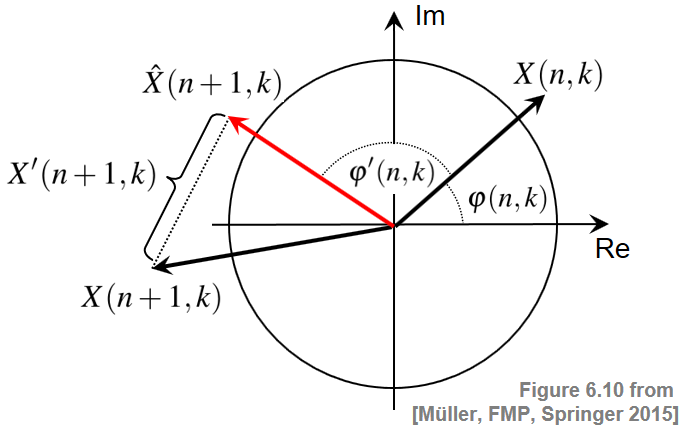
We have seen that steady regions within a signal may be characterized by a phase-based criterion in the case that the sinusoid correlates well with the signal. However, if the magnitude of the Fourier coefficient $\mathcal{X}(n,k)$ is very small, the phase $\varphi(n,k)$ may exhibit a rather chaotic behavior due to small noise-like fluctuations that may occur even within a steady region of the signal. To obtain a more robust detector, one idea is to weight the phase information with the magnitude of the spectral coefficient. This leads to a complex-domain variant of the novelty function, which jointly considers phase and magnitude. The assumption of this variant is that the phase differences as well as the magnitude stay more or less constant in steady regions. Therefore, given the Fourier coefficient $\mathcal{X}(n,k)$, one obtains a steady-state estimate $\hat{\mathcal{X}}(n+1,k)$ for the next frame by setting
\begin{eqnarray} \varphi'(n,k) &:=& \varphi(n,k)- \varphi(n-1,k), \\ \hat{\mathcal{X}}(n+1,k) &:=& |\mathcal{X}(n,k)|\,\, \mathrm{exp}(2\pi i(\varphi(n,k)+\varphi'(n,k))), \end{eqnarray}Then, we can use the magnitude between the estimate $\hat{\mathcal{X}}(n+1,k)$ and the actual coefficient $\mathcal{X}(n+1,k)$ to obtain a measure of novelty:
\begin{equation} \mathcal{X}'(n+1,k) = |\hat{\mathcal{X}}(n+1,k)-\mathcal{X}(n+1,k)|. \end{equation}The complex-domain difference $\mathcal{X}'(n,k)$ quantifies the degree of nonstationarity for frame $n$ and coefficient $k$. The following figure illustrates the definitions:
Complex-Domain Novelty Function
Note that this number does not discriminate between note onsets (energy increase) and note offsets (energy decrease). Therefore, we decompose $\mathcal{X}'(n,k)$ into a component $\mathcal{X}^+(n,k)$ of increasing magnitude and a component $\mathcal{X}^-(n,k)$ of decreasing magnitude:
\begin{eqnarray} \mathcal{X}^+(n,k) = \left\{ \begin{array}{cl} \mathcal{X}'(n,k) & \, \mbox{for $|\mathcal{X}(n,k)|>|\mathcal{X}(n-1,k)|$}\\ 0 & \, \mbox{otherwise,} \end{array} \right.\\ \mathcal{X}^-(n,k) = \left\{ \begin{array}{cl} \mathcal{X}'(n,k) & \, \mbox{for $|\mathcal{X}(n,k)|\leq |\mathcal{X}(n-1,k)|$}\\ 0 & \, \mbox{otherwise.} \end{array} \right. \end{eqnarray}A complex-domain novelty function $\Delta_\mathrm{Complex}$ for detecting note onsets can then be defined by summing the values $\mathcal{X}^+(n,k)$ over all frequency coefficients:
\begin{equation} \Delta_\mathrm{Complex}(n,k) = \sum_{k=0}^{K}\mathcal{X}^+(n,k). \end{equation}Similarly, for detecting general transients or note offsets, one may compute a novelty function using $\mathcal{X}'(n,k)$ or $\mathcal{X}^-(n,k)$, respectively.
Implementation
In the following code cell, one finds an implementation of this idea. As for the spectral-based novelty function, one may add further processing steps such as logarithmic compression of the magnitude, subtracting a local average, and normalization dividing the curve by its maximum value.
librosa.stft function in Python, the convention is reversed, and X[k,n] represents the corresponding Fourier coefficient. The differing conventions between theory and implementation can indeed introduce potential sources of errors, and it is essential to keep this in mind when translating theoretical concepts into practical code.
import numpy as np
import os, sys, librosa
from scipy import signal
from matplotlib import pyplot as plt
import IPython.display as ipd

sys.path.append('..')
import libfmp.b
import libfmp.c2
import libfmp.c6
from libfmp.c6 import compute_local_average

%matplotlib inline

def compute_novelty_complex(x, Fs=1, N=1024, H=64, gamma=10.0, M=40, norm=True):
    """Compute complex-domain novelty function

    Notebook: C6/C6S1_NoveltyComplex.ipynb

    Args:
        x (np.ndarray): Signal
        Fs (scalar): Sampling rate (Default value = 1)
        N (int): Window size (Default value = 1024)
        H (int): Hop size (Default value = 64)
        gamma (float): Parameter for logarithmic compression (Default value = 10.0)
        M (int): Determines size (2M+1) in samples of centric window used for local average (Default value = 40)
        norm (bool): Apply max norm (if norm==True) (Default value = True)

    Returns:
        novelty_complex (np.ndarray): Energy-based novelty function
        Fs_feature (scalar): Feature rate
    """
    X = librosa.stft(x, n_fft=N, hop_length=H, win_length=N, window='hanning')
    Fs_feature = Fs / H
    mag = np.abs(X)
    if gamma > 0:
        mag = np.log(1 + gamma * mag)
    phase = np.angle(X) / (2*np.pi)
    phase_diff = np.diff(phase, axis=1)
    phase_diff = np.concatenate((phase_diff, np.zeros((phase.shape[0], 1))), axis=1)
    X_hat = mag * np.exp(2*np.pi*1j*(phase+phase_diff))
    X_prime = np.abs(X_hat - X)
    X_plus = np.copy(X_prime)
    for n in range(1, X.shape[1]):
        idx = np.where(mag[:, n] < mag[:, n-1])
        X_plus[idx, n] = 0
    novelty_complex = np.sum(X_plus, axis=0)
    if M > 0:
        local_average = compute_local_average(novelty_complex, M)
        novelty_complex = novelty_complex - local_average
        novelty_complex[novelty_complex < 0] = 0
    if norm:
        max_value = np.max(novelty_complex)
        if max_value > 0:
            novelty_complex = novelty_complex / max_value
    return novelty_complex, Fs_feature

fn_ann = os.path.join('..', 'data', 'C6', 'FMP_C6_F01_Queen.csv')
ann, label_keys = libfmp.c6.read_annotation_pos(fn_ann)

fn_wav = os.path.join('..', 'data', 'C6', 'FMP_C6_F01_Queen.wav')
Fs = 22050
x, Fs = librosa.load(fn_wav, Fs)
x_duration = len(x)/Fs

nov, Fs_nov = compute_novelty_complex(x, Fs=Fs, gamma=10, M=0, norm=1)
fig, ax, line = libfmp.b.plot_signal(nov, Fs_nov, color='k',
                    title='Complex-domain novelty function')
libfmp.b.plot_annotation_line(ann, ax=ax, label_keys=label_keys,
                    nontime_axis=True, time_min=0, time_max=x_duration);

nov, Fs_nov = compute_novelty_complex(x, Fs=Fs, gamma=10, M=40, norm=1)
fig, ax, line = libfmp.b.plot_signal(nov, Fs_nov, color='k',
                    title='Complex-domain novelty function with post-processing')
libfmp.b.plot_annotation_line(ann, ax=ax, label_keys=label_keys,
                    nontime_axis=True, time_min=0, time_max=x_duration);


Further Notes
- In the FMP notebook on onset detection, one finds an introduction to the task of onset detection.
- In the FMP notebook on novelty comparison, we compare different novelty detection approaches.
 |
 |
 |
 |
 |
 |
|
 |
 |