Music Synchronization

In this notebook, we give an example for music synchronization following Chapter 3 of [Müller, FMP, Springer 2015]. For technical details we refer to Section 3.1 (Audio Features) and Section 3.2 (Dynamic Time Warping).

Introduction

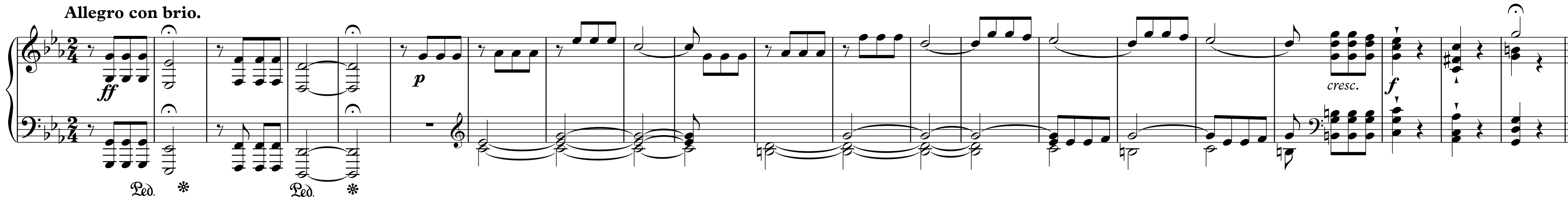
Music can be described and represented in many different ways including sheet music, symbolic representations, and audio recordings. For each of these representations, there may exist different versions that correspond to the same musical work. For example, for Beethoven's Fifth Symphony one can find a large number of music recordings performed by different orchestras and conductors. As our main example in this notebook, we consider the beginning of Beethoven's Fifth Symphony (first 21 measures) as shown below in form of a piano-reduced version (for a full score, we refer to the FMP notebook on Sheet Music Representations. Let us listen to two different recordings. The first recording is a synthesized version of a piano-reduced score, whereas the second recording is an interpretation by the Vienna Philharmonic Orchestra conducted by Herbert von Karajan, 1946.

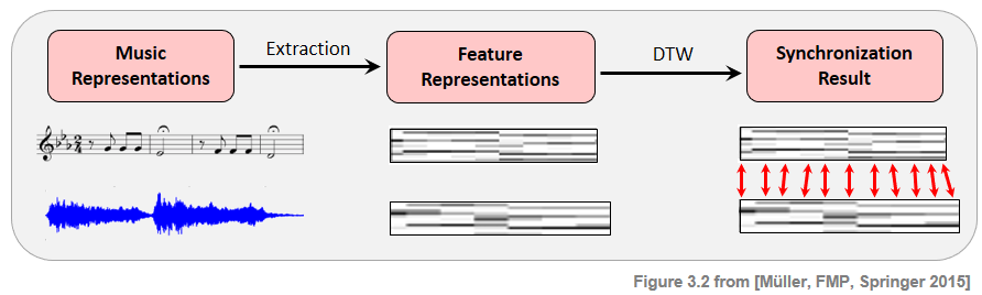
Given two different music representations, typical synchronization approaches proceed in two steps.

• In the first step, the two representations are transformed into sequences of suitable features. In general, such feature representations need to find a compromise between two conflicting goals. On the one hand, features should show a large degree of robustness to variations that are to be left unconsidered for the task at hand. On the other hand, features should capture enough characteristic information to accomplish the given task. In the following, we use chroma-based features, which capture harmonic and melodic characteristics of music, while being robust to changes in timbre and instrumentation.

• In the second step, the derived feature sequences have to be brought into temporal correspondence. To this end, one may use dynamic time warping (DTW) for computes an optimal alignment between two given feature sequences. This alignment constitutes our synchronization result.

The following figure gives an overview of this two-step processing pipeline.

Chroma-Based Feature Representation

To compare the two recordings, we convert the audio signals into sequences of chroma vectors. In the following, we use the Python package librosa to load and process the audio recordings. Starting with the sampling rate $F_\mathrm{s}=22050$ Hz, we use an STFT using a window length of $N=4410$ and a hop size of $H=2205$ samples. This results in feature sequences of $10$ features per seconds (feature resolution of $10$ Hertz). Furthermore, the chroma features are normalized with respect to the $\ell^2$-norm.

import os
import numpy as np
import matplotlib.pyplot as plt
import IPython.display as ipd
import librosa, librosa.display
%matplotlib inline

import sys
sys.path.append('..')
import libfmp.c3

Fs = 22050
fn_wav_X = os.path.join('..', 'data', 'C3', 'FMP_C3S3_Beethoven_Fifth-MM1-21_Midi-Piano.wav')
fn_wav_Y = os.path.join('..', 'data', 'C3', 'FMP_C3S3_Beethoven_Fifth-MM1-21_Karajan1946.wav')
X_wav, Fs = librosa.load(fn_wav_X, sr=Fs)
Y_wav, Fs = librosa.load(fn_wav_Y, sr=Fs)

N = 4410
H = 2205
X = librosa.feature.chroma_stft(y=X_wav, sr=Fs, tuning=0, norm=2, hop_length=H, n_fft=N)
Y = librosa.feature.chroma_stft(y=Y_wav, sr=Fs, tuning=0, norm=2, hop_length=H, n_fft=N)

plt.figure(figsize=(8, 2))
plt.title('Sequence $X$')
librosa.display.specshow(X, x_axis='frames', y_axis='chroma', cmap='gray_r', hop_length=H)
plt.xlabel('Time (frames)')
plt.ylabel('Chroma')
plt.colorbar()
plt.clim([0, 1])
plt.tight_layout(); plt.show()
ipd.display(ipd.Audio(X_wav, rate=Fs))

plt.figure(figsize=(8, 2))
plt.title('Sequence $Y$')
librosa.display.specshow(Y, x_axis='frames', y_axis='chroma', cmap='gray_r', hop_length=H)
plt.xlabel('Time (frames)')
plt.ylabel('Chroma')
plt.colorbar()
plt.clim([0, 1])
plt.tight_layout(); plt.show()
ipd.display(ipd.Audio(Y_wav, rate=Fs))