
Overview and Learning Objectives
Python has several useful built-in packages as well as additional external packages. One such package is NumPy, which adds support for multi-dimensional arrays and matrices, along with a number of mathematical functions to operate on these structures. This unit covers array objects as the most fundamental NumPy data structure along with important NumPy array operations. Furthermore, we discuss numerical types, methods for type conversion, and constants (including the constants nan and inf) offered by NumPy. The three exercises included at the end of this unit cover key aspects needed throughout the PCP notebooks. Therefore, we encourage students to work through these exercises carefully. In particular, we recapitulate the mathematical concept of matrices and matrix multiplication, before we cover these aspects in Exercise 2 from an implementation perspective. We believe that understanding both—the mathematical formulation of abstract concepts and their realization in a programming context—is key in engineering education. This philosophy also forms the basis of the PCP notebooks to follow.
NumPy Module
As said above, NumPy is a Python library used for working with arrays. In principle, one can also use the Python concept of lists to model an array. However, processing such lists is usually slow. Being mostly written in C or C++ and storing arrays at continuous places in memory (unlike lists), NumPy can process and compute with arrays in a very efficient way. This is the reason why NumPy is so powerful. In order to use NumPy, one needs to install the numpy package. This is what we already did when we created the PCP Environment, which contains a numpy-version. Furthermore, we need to use the Python import statement to get access to the NumPy functions. It is convenient to assign a short name to a frequently-used package (for example np in the case of numpy). This short name is used as a prefix when calling a function from the package. In the following code cell, we import numpy as np. To find out what the numpy-module contains, we use the Python command dir(np) to return a list all properties and methods of the specified module.
import numpy as np
list_numpy_names = dir(np)
print(list_numpy_names)
NumPy Arrays
The fundamental NumPy data structure is an array object, which represents a multidimensional, homogeneous array of fixed-size items. Each array has a shape, a type, and a dimension. One way to create a NumPy array is to use the array-function. In the following code cells, we provide various examples and discuss basic properties of NumPy arrays.
import numpy as np

x = np.array([1, 2, 3, 3])
print('x = ', x)
print('Shape:', x.shape)
print('Type:', x.dtype)
print('Dimension:', x.ndim)
Note that, in this example, x.shape produces a one-element tuple, which is encoded by (4,) for disambiguation. (The object (4) would be an integer of type int rather than a tuple.) Two-dimensional arrays (also called matrices) are created like follows:
x = np.array([[1, 2, 33], [44, 5, 6]])
print('x = ', x, sep='\n')
print('Shape:', x.shape)
print('Type:', x.dtype)
print('Dimension:', x.ndim)
There are a couple of NumPy functions for creating arrays:
print('Array of given shape and type, filled with zeros: ', np.zeros(2))
print('Array of given shape and type, filled with integer zeros: ', np.zeros(2, dtype='int'))
print('Array of given shape and type, filled with ones: ', np.ones((2, 3)), sep='\n')
print('Evenly spaced values within a given interval: ', np.arange(2, 8, 2))
print('Random values in a given shape: ', np.random.rand(2, 3),  sep='\n')
print('Identity matrix: ', np.eye(3),  sep='\n')
Array Reshaping
Keeping the total number of entries, there are various ways for reshaping an array. Here are some examples:
x = np.arange(2 * 3 * 4)
print('x =', x)
print('Shape:', x.shape)

y = x.reshape((3, 8))
print('y = ', y, sep='\n')
print('Shape:', y.shape)

z = np.reshape(x, (3, 2, 4))
print('z = ', z, sep='\n')
print('Shape:', z.shape)

print('Element z[0, 1, 2] = ', z[0, 1, 2])
NumPy allows for giving one of the new shape parameters as -1. In this case, NumPy automatically figures out the unknown dimension. Note the difference between the shape (6,) and the shape (6,1) in the following example.
x = np.arange(6)
print(f'Shape: {x.shape}; dim: {x.ndim}')
x = x.reshape(-1, 2)
print(f'Shape: {x.shape}; dim: {x.ndim}')
x = x.reshape(-1, 1)
print(f'Shape: {x.shape}; dim: {x.ndim}')
Array Operations
There are many ways to compute with NumPy arrays. Many operations look similar to the ones when computing with numbers. Applied to arrays, these operations are conducted in an element-wise fashion:
x = np.arange(5)
print('x = ', x)
print('x + 1 =', x + 1)
print('x * 2 =', x * 2)
print('x * x =', x * x)
print('x ** 3 =', x ** 3)
print('x / 4 =', x / 4)
print('x // 4 =', x // 4)
print('x > 2 =', x > 2)
Here are some examples for computing with matrices of the same shape. It is important to understand the difference between element-wise multiplication (using the operator *) and usual matrix multiplication (using the function np.dot):
a = np.arange(0, 4).reshape((2, 2))
b = 2 * np.ones((2, 2))
print('a = ', a, sep='\n')
print('b = ', b, sep='\n')
print('a + b = ', a + b, sep='\n')
print('a * b (element-wise multiplication) = ', a * b, sep='\n')
print('np.dot(a, b) (matrix multiplication) = ', np.dot(a, b), sep='\n')
Note that arrays and lists may behave in a completely different way. For example, using the operator + leads to the following results:
a = np.arange(4)
b = np.arange(4)
print(a + b, type(a + b))

a = list(a)
b = list(b)
print(a + b, type(a + b))
The sum of an array's elements can be computed along the different dimensions specified by the parameter axis. This is illustrated by the following example:
x = np.arange(6).reshape((2, 3))
print('x = ', x, sep='\n')
print('Total sum:', x.sum())
print('Column sum: ', x.sum(axis=0))
print('Row sum:', x.sum(axis=1))
There are many ways for accessing and manipulating arrays. Here are some examples:
x = np.arange(6).reshape((2, 3))
print('x = ', x, sep='\n')
print('Element in second column of second row:', x[1, 1])
print('Boolean encoding of element positions with values larger than 1: ', x > 1, sep='\n')
print('All elements larger than 1:', x[x > 1])
print('Second row:', x[1, :])
print('Second column:', x[:, 1])
NumPy Type Conversion
In the PCP Notebook on Python Basics, we have already discussed the standard numeric types int, float, and complex offered by Python (and the function type() to identify the type of a variable). The NumPy package offers many more numerical types and methods for type conversion. We have already seen how to obtain the type of a numpy array using dtype. One can create or convert a variable to a specific type using astype. Some examples can be found in the next code cell.
a = np.array([-1,2,3])
print(f'a = {a}; dtype: {a.dtype}')
b = a.astype(np.float64)
print(f'b = {b}; dtype: {b.dtype}')
c = a.astype(np.int64)
print(f'c = {c}; dtype: {c.dtype}')
d = a.astype(np.uint8)
print(f'd = {d}; dtype: {d.dtype}')
e = np.array([1,2,3]).astype(np.complex64)
print(f'e = {e}; dtype: {e.dtype}')
Specifying the exact type is often important when using packages such as numba for optimizing machine code at runtime. In the following example, we give an example where a wrong initialization leads to an error (or warning with some nan results) when computing the square root of a negative number.
print('=== Initialization with \'int32\' leading to an error ===', flush=True)
x = np.arange(-2, 2)
print(x, x.dtype)
x = np.sqrt(x)
print(x)

print('=== Initialization with \'complex\' ===', flush=True)
x = np.arange(-3, 3, dtype='complex')
print(x, x.dtype)
x = np.sqrt(x)
print(x)
NumPy Constants
NumPy offers several constants that are convenient to compute with. In the following, we give some examples:
print(f'Archimedes constant Pi: {np.pi}; type: {type(np.pi)}')
print(f'Euler’s constant, base of natural logarithms: {np.e}; type: {type(np.e)}')
print(f'Floating point representation of (positive) infinity: {np.inf}; type: {type(np.inf)}')
print(f'Floating point representation of (negative) infinity: {-np.inf}; type: {type(-np.inf)}')
print(f'floating point representation of Not a Number (NaN): {np.nan}; type: {type(np.nan)}')
In particular, the constants nan and inf can be convenient to avoid case distinctions. However, computing with such constants can also be a bit tricky as the following examples show.
a = 10
b = np.inf
c = -np.inf
d = np.nan

print(f'a = {a}, b = {b}, c = {c}, d = {d}')
print('a + b =', a + b)
print('a * b =', a * b)
print('a + c =', a + c)
print('a - c =', a - c)
print('a + d =', a + d)
print('b + c =', b + c)
print('b * c =', b * c)
print('b / c =', b / c)
print('b + d =', b + d)
NumPy offers functions such as np.where and np.isinf to check for special constants. In the following, the class np.errstate is used to suppress warning that are usually output when dividing by zero.
print('Test element-wise for positive or negative infinity:', np.isinf([np.inf, -np.inf, np.nan]))

a = np.arange(-2, 3)
print('a = ', a)
with np.errstate(divide='ignore', invalid='ignore'):
    b = a / 0
print('b = a / 0 =', b)

ind_inf = np.isinf(b)
ind_inf_pos = np.where(ind_inf)
print('Indices with inf values:', ind_inf, ind_inf_pos)

ind_nan = np.isnan(b)
ind_nan_pos = np.where(ind_nan)
print('Indices with nan values:', ind_nan, ind_nan_pos)
Exercises and Results
import libpcp.numpy
show_result = True
- Create a NumPy array
awith ascending natural numbers in the interval $[10, 20]=\{10,11,\ldots,20\}$ (usingnp.arange). - Set all entries of
ato zero wherea$\leq13$ anda$>16$. - Extend the resulting array
awith a NumPy array containing the numbers of the interval $[4,6]$ and store the result in a variableb(usingnp.append). - Remove duplicate values of
b(usingnp.unique) and store the result in a variablec. Note that the result is automatically sorted in ascending order. - Sort
cin descending order and store the result in a variabled. Explore and discuss various options to do this including the slicing methodc[::-1], the functionreversed(), as well as the NumPy functionsnp.sortandnp.flip.
#<solution>
# Your Solution
#</solution>
libpcp.numpy.exercise_numpy_array(show_result=show_result)
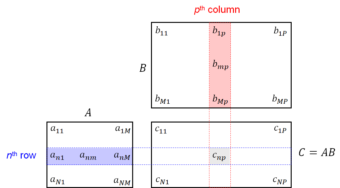
Let $N,M\in\mathbb{N}$ be two positive integers. An $(N\times M)$-matrix $\mathbf{A}$ is a rectangular array of entries arranged in rows and columns. For example, if entries are real numbers, one also writes $\mathbf{A}\in\mathbb{R}^{N\times M}$. Let $a_{nm}\in\mathbb{R}$ denote the entry of $\mathbf{A}$ being in the $n^{\mathrm{th}}$ row and $m^{\mathrm{th}}$ column for $n\in[1:N]=\{1,2,...,N\}$ and $m\in[1:M]$. Then, one also often writes $\mathbf{A}=[a_{nm}]$. A vector is a matrix where either $N=1$ (then called row vector) or $M=1$ (then called column vector).
When computing with vectors and matrices, one has to pay attention that the dimensions $N$ and $M$ of the operands match properly. For example, for a matrix summation or matrix subtraction, the operands must be of same dimensions or one of them needs to be a scalar (in this case the operations are applied per entry). The multiplication of matrices refers to a matrix multiplication. For an $(N\times M)$-matrix $\mathbf{A} = [a_{nm}]$ and a $(M\times P)$-matrix $\mathbf{B} = [b_{mp}]$, the product matrix $\mathbf{C} = \mathbf{A}\mathbf{B}$ with entries $\mathbf{C}=[c_{np}]$ is defined by $c_{np} = \sum_{m=1}^M a_{nm}b_{mp}$ for $n\in[1:N]$ and $p\in[1:P]$. In other words, the entry $c_{np}$ is the inner product (sometimes also called scalar product) of $n^{\mathrm{th}}$ row of $\mathbf{A}$ and $p^{\mathrm{th}}$ column of $\mathbf{B}$. This calculation rule is illustrated by the following figure:
- Construct a matrix $\mathbf{B} = \begin{bmatrix}2 & 2 & 2 & 2\\2 & 2 & 2 & 2\\0 & 0 & 0 & 0\\\end{bmatrix}$ just using the NumPy functions
np.zeros,np.ones, andnp.vstack. Check the matrix dimensions usingnp.shape. - Find the row and column index of the maximum entry of the matrix $\mathbf{D} = \begin{bmatrix}2 & 0 & 2\\-1 & 5 & 10\\-3 & 0 & 9\\\end{bmatrix}$ using the functions
np.max,np.argmaxandnp.unravel_index. Why is it not sufficient to usenp.argmax? - Given a row vector $\mathbf{v} = [3\;2\;1]$ and a column vector $\mathbf{w} = [6\;5\;4]^T$, compute $\mathbf{v}\mathbf{w}$ and $\mathbf{w}\mathbf{v}$ using
np.dotandnp.outer. What is the difference betweennp.multiply,np.dot, andnp.outer? - Given $\mathbf{A} = \begin{bmatrix}1 & 2\\3 & 5\end{bmatrix}$, $\mathbf{v} = \begin{bmatrix}1\\4\end{bmatrix}$, compute $\mathbf{A}^{-1}$ and $\mathbf{A}^{-1}\mathbf{v}$ (using
np.linalg.inv).
#<solution>
# Your Solution
#</solution>
libpcp.numpy.exercise_matrix_operation(show_result=show_result)
The NumPy package offers many different mathematical functions. Explore these functions by trying them out on small examples. In particular, you should gain a good understanding of the following concepts.
- Generate a NumPy array
v_degcontaining the numbers $[0, 30, 45, 60, 90, 180]$. Apply the functionnp.deg2radto convert this array (given in degree) to an arrayv_rad(given in radiants). Then apply the functionsnp.cosandnp.sinand discuss the results. - Using the the same array as before, apply the exponential function
np.exp(1j * v_rad). What is meant by1j? What is the relation tonp.cosandnp.sin? Use the functionsnp.real,np.imag, andnp.iscloseto make this relation explicit. - Try out different functions for rounding using the numbers $[-3.1416, -1.5708, 0, 1.5708, 3.1416]$. What is the difference between the functions
np.round,np.floor,np.ceil, andnp.trunc?
#<solution>
# Your Solution
#</solution>
libpcp.numpy.exercise_numpy_math_function(show_result=show_result)
